A bizarre series of events in a college microbiology lab class left 33 people—including students, professors, and lab workers—believing they were exposed to a deadly germ. Of those, 32 began taking an antibiotic regimen as a precaution to prevent a life-threatening infection. Two also underwent lumbar punctures—aka spinal taps—after developing mild symptoms.
But none of them had actually been exposed to a dangerous pathogen, a fortunate twist in the strange incident, which otherwise stands to be a cautionary tale for the ages. The incident was published in a recent issue of Morbidity and Mortality Weekly Report.
It began with a simple laboratory exercise. The microbiology lab students were supposed to be given mystery bacteria by their instructors and then identify the microbe based on a series of biochemical tests and morphological characterization.
Please Use AI. “Be sure to use AI when planning that next camping trip, the last one you will take with this particular child. Definitely do not text your friend who has fly-fished every river in Pennsylvania and biked every backwoods trail…”
Like all American children, I spent a week of each school year learning to sculpt a largemouth bass out of clay.
I cannot tell you why this was part of the annual curriculum at Perry Elementary School, nor why it started in first grade. At that age, I’m not sure any of my classmates had ever seen a largemouth bass; they may as well have asked us to sculpt a particle collider. I can only tell you the results were predictable. My first bass was a cursed, torturous creature, mostly mouth by volume. It looked like someone had tried to turn a fish inside out and gotten bored halfway through.
Still, I thought I could rescue it with design. The school had given us tempera paint in fluorescent colors, but I was hell-bent on creating something new. I stirred the Day-Glo pinks and greens together and watched them collapse into a muddy brown—the dusty, dull brown of a moose without a skincare regimen. I was delighted. My art teacher wasn’t.
This was when I first learned to think of complexity as an aesthetic burden, a lesson I’d be re-taught in almost every creative field. To let colors (sounds, flavors) shine, conventional wisdom dictated, you had to keep things simple.
The year I shaped my first bass was also the year I sipped my first “suicide”—the slang term for mixing all of the flavors at the soda fountain into a single plastic cup.1 Perhaps you know it by that name, or by another equally disturbing one. Some people call the soda a “kamikaze”; in pockets of the Pacific Northwest, it’s better known as a “graveyard.” The exact etymology is fuzzy—it’s not clear which term came first—but it’s death spirals all the way down.
The terms are also surprisingly old. In my research, I found references to both “suicides” and “graveyards” starting in 1950. In the same year the Detroit Free Press referenced a “graveyard soda,” the Akron Beacon Journal published a note about “suicide sodas” that was ostensibly a trend piece but actually an excuse to publish feet pics.
We love to sip soda at Drugstore!
It’s tempting to think of the suicide as a novelty or a gimmick. But I’m not sure kids would still be drinking them 75 years later if that was their only appeal. My memory of childhood suicides—there’s a setup that will get my mother to call—is of a soda that defied the aesthetic principles I was only just starting to absorb. I remember a soda that stayed pleasant and drinkable even as it was tugged in a dozen different directions. I remember a soda that was, if not greater than, at least equal to the sum of its parts.
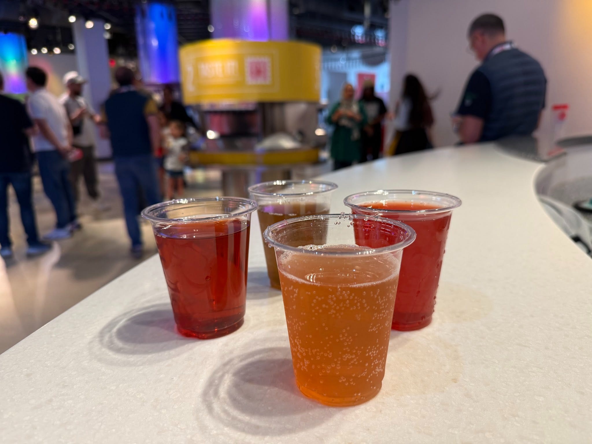
But like a child sculpting a largemouth bass, I wanted to know what would happen if I added one part too many. So in April, I flew to Atlanta to visit the World of Coca-Cola, an innovative museum where customers pay to see advertisements. The main draw (for me, at least) was Taste It!, a very sticky library of more than 100 different soda flavors. The room was a United Nations Assembly of fountain beverages, from Peru’s bubblegum-adjacent Inca Kola to China’s Fanta Sour Plum, which tastes like Liquid Smoke and cabinet hinges, to Zimbabwe’s Sparletta Sparberry, a surrealist soda designed to showcase the flavor of an imaginary fruit.
But the marquee attraction for irredeemable soda jerks is “Beverly.” Beverly is an aperitif-aping Italian soda that’s become infamous not only for its name but for its flavor, which I would describe with great affection as “carbonated Malört.” You will be unsurprised to hear that I loved Beverly and consumed several glasses of Her before refocusing on my mission: creating the world’s largest, most inclusive suicide.
I quickly ran into a predictable constraint: It is impossible to fit even the merest splashes of 100 different sodas into a single 8-ounce cup. In the end, I needed four cups to collect all my samples. I combined them into a fifth cup by furiously decanting them back and forth like some sort of carnival mixologist.
The result was an affront to received wisdom. The ultimate suicide—I’m calling it the “International Incident”—wasn’t muddy. It was complex. It tasted like a lychee cream soda with floral, jasmine-y notes and a surprisingly bitter backbone. There was a little raspberry, a little Beverly, a little plum. I liked it better than most of the sodas in isolation. I liked it better than most sodas.
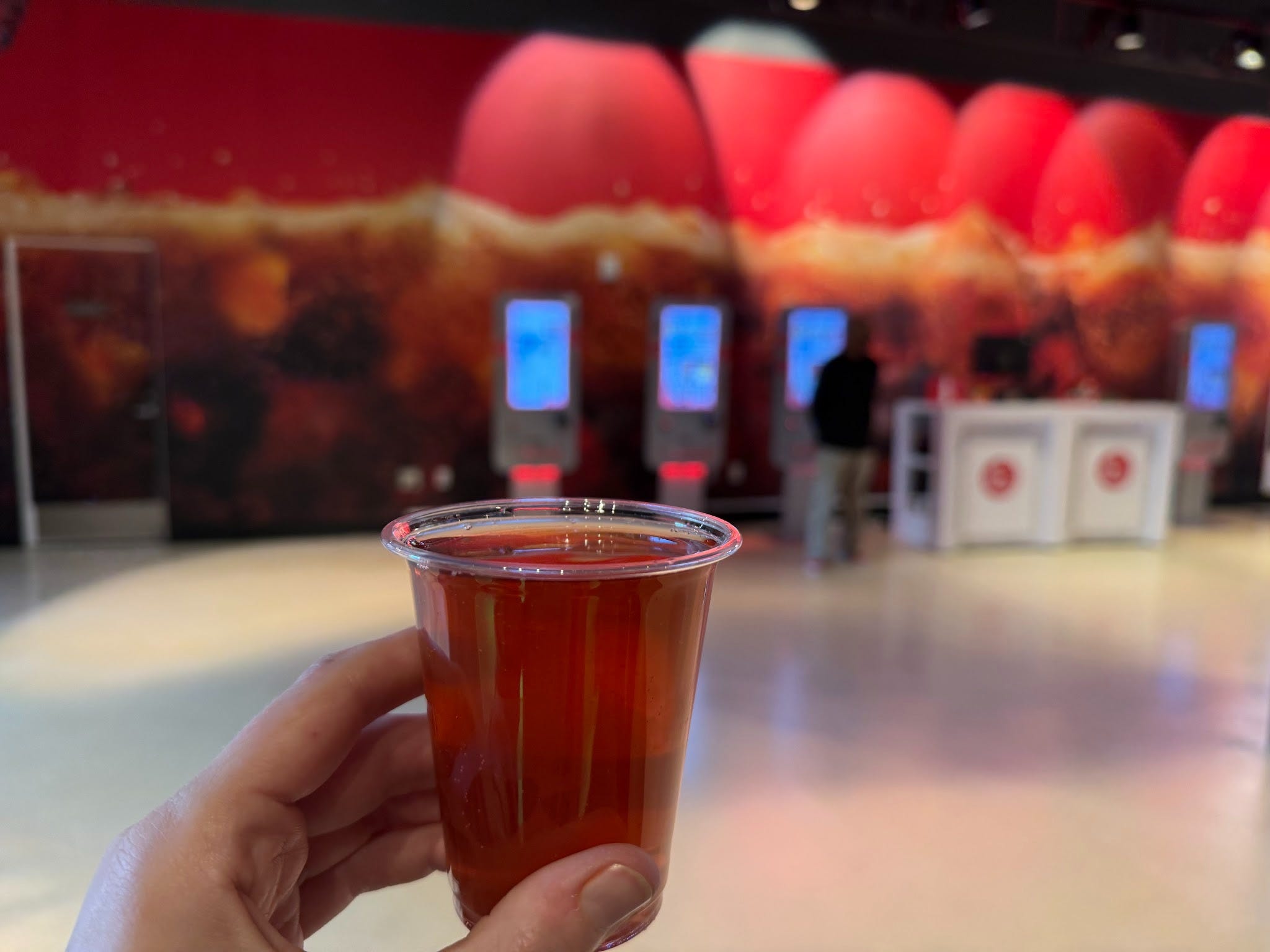
Even the color was surprising—a deep red, the devil’s hue.2 It seemed implausible that 100 sodas mixed together could yield a vibrant, primary color. I can only assume there is an ancient color memory hidden deep within sugar molecules. The soda yearns to be red.
For reasons that have nothing to do with my soda consumption, I’ve started waking up at 3 AM most days with a mounting feeling of unspecified dread. At first, I tried to fight it by purchasing a soft, lavender-stuffed goose that I could heat in the microwave. But Goosetace didn’t fix the problem, and I have since given up tacking against the feeling. I now spend my too-early mornings reading about dismal subjects like “redshift”—the cosmological color of objects moving away from us as our universe expands. As stars and galaxies hurtle ever farther from Earth, their light stretches out to us in longer, redder wavelengths.3 Redshift is inherently lonely. It’s a visual reminder that the rest of the universe can’t wait to get away.
The International Incident at the World of Coca-Cola introduced me to the opposite of redshift—a ruby-red tint created not by distance, but by proximity. Blending 100 different sodas together is an insane act, but it’s also a hopeful one. Conventional wisdom says it shouldn’t work. It does, anyway.
I suspect my elementary school art teachers may have gotten a few things wrong, though my bass technique is vastly improved. I don’t think complexity is an aesthetic burden any more than I think simplicity is an aesthetic gift. Overdoing it and underdoing it have the same moral weight. And we’ve erred in favor of simplicity and specialization long enough.
It’s time to embrace the sunny side of the suicide: an invitation to a busier, more crowded Age. It is time to embrace chaos—to embrace doing nothing well and a lot of things poorly. It is time to paint the largemouth bass in moose-y neutrals. To grind all the spices together. To name an ice cream flavor “Chris.”4
The rest of the universe is on the lam; the clutter of this world might be all we have to work with. Humanity is a messy, sticky, destructive business, but it’s the only one I want to be in.
Haterade is a free newsletter sustained by angry astrophysicists and prepubescent anglers. The best way to support the newsletter is to share it! If you’d like to help fund the Liz Cook Center for Ceramic Fish Arts, become apaid subscriber(never a perk, always a thrill) or stuff some money in the tip jar here: Venmo | PayPal.
I spent my summers at Vacation Bible School, a place where parents who can’t afford summer camp send their children to be rid of them. Every year, for Religious Reasons, we mixed glitter and various fluids inside a plastic water bottle to create an oily blue ocean. This, like the large-mouthed bass, was intended as a Gift for our parents. Do not ask me what the Gift was meant to represent. I do not remember most of the things I was supposed to learn at Bible School—What is an Ephesian? Is it good?—but I do remember that Blue Liquid brings us closer to God.
My friend Ben is an astrophysicist, and he will hate this whole paragraph. If I were an astrophysicist, I would also be tired of writers misrepresenting scientific principles for their metaphors. As a gesture of goodwill, I invite the astrophysics community to turn the Haterade of their choice into math.
Note from Emily and Denise: We are noticing that EdTech companies seem to be shifting uncomfortably in their metaphorical chairs these days— increasingly so as the school year approaches and concerns about their products’ presence in schools grows. We believe we are witnessing an “EdTech industry rebrand” and we’re here to call it out. This is Part 1 of a two-part essay.
In response, instead of pulling their health-harming products from the classrooms or seeking external audits and independently verifiable scientific research to prove their claims, they’re getting a makeover.
But the trouble is, “Children do not need tech; technology companies need children,” as Emily pointed out recently in her testimony to the Kentucky State Senate on education and screentime. At the end (and beginning) of the day, EdTech is an industry– a massive one worth nearly $200 billion currently, with some projections putting it at nearly double that over the next ten years. (Can you imagine if schools had budgets like that?)
“How do we grow when the easy money is gone?”
EdTech products are heavily pushed into school districts by an industry that is well-funded and skilled at marketing. As one example (and there are many), the Tech & Learning EdExec Summit scheduled for September 2026 is pitched to attract:
CEOs & Founders “who need to steer the ship through economic uncertainty”;
Sales & Marketing Directors “who need to shorten complex sales cycles and bypass gatekeepers”;
Product Managers “who need to build for ‘Evidence-Based’ compliance and interoperability”; and
Strategic Partnership Directors/Business Development “looking to build relationships with key industry players.”
This “learning” summit promises that attendees will have access not just to industry executives, but “school district administrators” too.
The “two-day strategic summit” will seek to answer one question: “How do we grow when the easy money is gone?”
The hosts of the Tech & Learning EdExec Summit say the experience is built to “deconstruct the real friction points in today’s district sales cycle—guided by the leaders who control the budgets.“ Attendees will “get valuable insight into the education market in time for the Back-to-School buying season.” Who are these attendees?
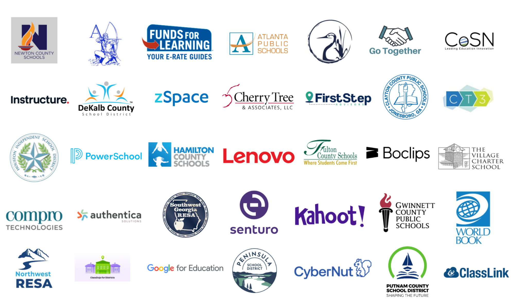
Here’s a list:
Who attends the Tech & Learning EdExec Summit? Lots of companies who stand to profit from potential business deals!
It seems to us that the only “learning” occurring here is how to keep milking the cow even when she’s gone dry.
The problem is the business model of the EdTech companies.
These companies rely on “time on device” and “engagement” to compete for a piece of that $200 billion pie, but this business model is fundamentally in opposition to healthy child development.
The problem is the business model of the EdTech companies. These companies rely on “time on device” and “engagement” to compete for a piece of a $200 billion pie, but this business model is fundamentally in opposition to healthy child development.
It doesn’t matter if an EdTech company has a noble mission, or if they have high quality materials, or if they swear they do not collect and sell student data— at the end of the day, if their business model depends on children spending time on a device this is no different than the business models of social media companies.
That’s why we say “EdTech is just Big Tech in a sweater vest”— the business models of Instagram and Snap and Meta are the same as iReady and Seesaw and Canvas. (Which may explain why Emily is also finding she has to fight to protect her intellectual property and trademarks from being co-opted by the very industry she is battling.)
This is how we find ourselves in the middle of Extreme Makeover: EdTech Edition.
The EdTech Industry’s New Look: “Purpose-Built EdTech”
The EdTech industry has taken notice of our movement…and they are concerned. They’re seeing and feeling the impact (and trolling us on social media). They are trotting out the same tired talking points that we’ve come to expect.
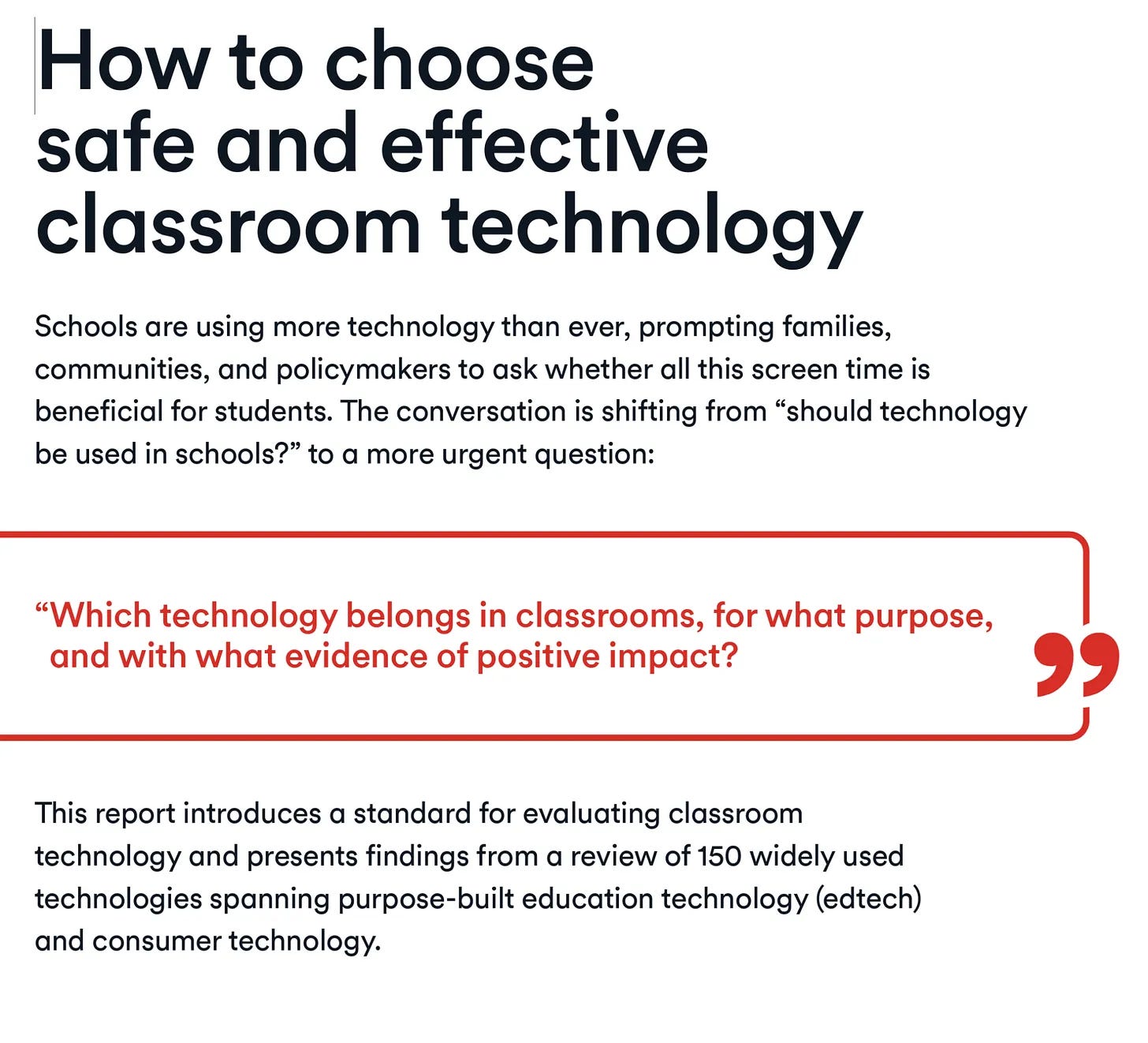
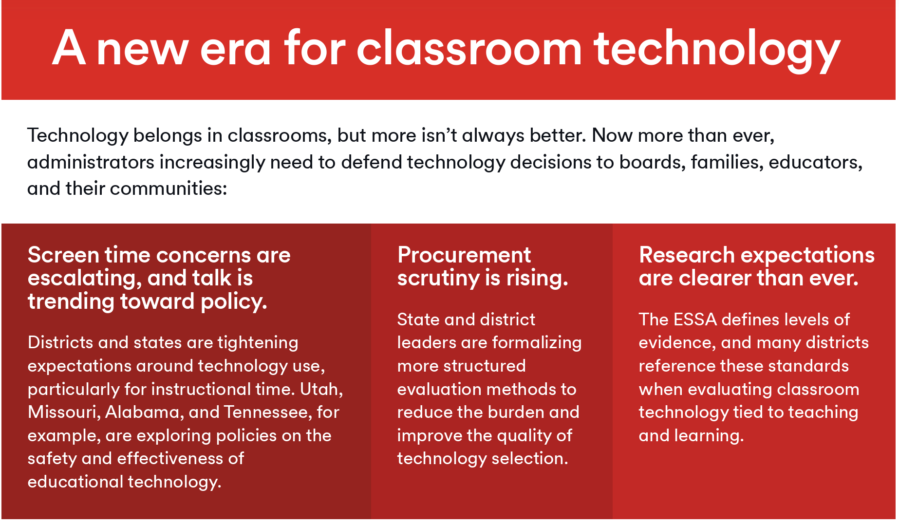
Instructure’s newest report claims to have analyzed the evidence, compliance and interoperability, and accessibility and usability of the top 150 EdTech products used in K-12 schools during Fall 2025. Before we dive into their report, we should point out that Instructure’s partnerships with companies like Google and Microsoft render such a “report” as scientifically compromised.
According to Instructure, “families, communities, and policymakers” are starting to ask if “all this screen time is beneficial for students.”
Screenshot from Instructure’s report
As a result of these questions being asked, Instructure believes, school leaders will need to defend their use of technology in the classroom to “boards, families, educators, and their communities.”
Of course, the most burning question is “Why weren’t they doing this before?”
Screenshot from Instructure’s report
Instructure, of course, has a “solution”: school leaders should make a distinction between “purpose-built” screentime and “consumer products,” and be sure parents and policymakers see Instructure products as the former not the later.
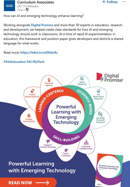
By attempting to put distance between “purpose-built EdTech” (which Instructure claims includes Kahoot! and iReady) and “Consumer Tech” (YouTube and ChatGPT), Instructure attempts to weave a story that “purpose-built” products like these offer more evidence of effectiveness and are safer.
Screenshot of LinkedIn post by Curriculum Associates
The only problem is that Digital Promise, an organization that describes itself as “a global nonprofit working to expand opportunity for every learner,” has numerous funders and partners with the tech industry.1
Emily and Denise were both lead authors on Fairplay’s recent Call for a Pause on AI in PreK-12th Grade and we firmly oppose the use of any AI products in education. We reject the notion that in an era of “rapid AI experimentation” that a “framework” given out by tech-funded “non-profit” and bestowed by a problematic EdTech company facing lawsuits for taking kids’ data without parental consent should be the arbiters of such designations.
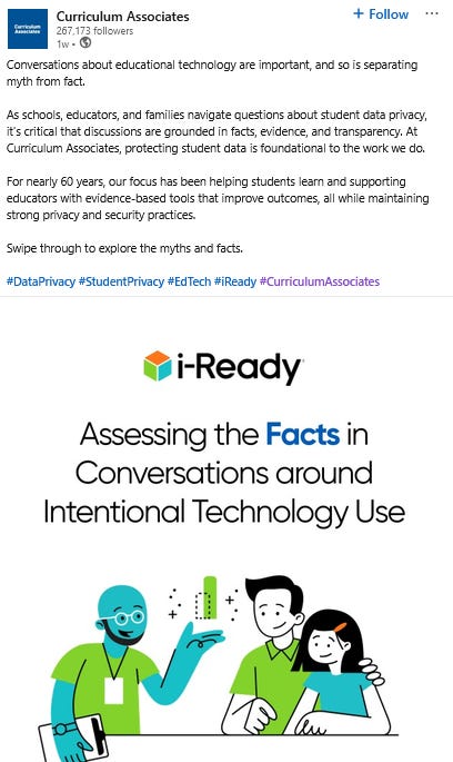
At the same time, the language now being used by Curriculum Associates (and other EdTech companies) sounds very similar to the “Tech-Intentional” framework created by Emily. We’re seeing this in multiple places, and as Emily has written about, it appears to be a growing issue.
Screenshot of a LinkedIn post by Curriculum Associates
It’s Not just EdTech Companies. It’s the Organizations Who Defend Them, Too.
We have written previously about the need to follow the money, not just behind EdTech companies, but the organizations that defend them, too.
One well-known example is ISTE, formerly the International Society for Technology in Education, who merged with ASCD (the Association for Supervision and Curriculum Development) in 2022 and recently rebranded themselves as the International Society for Transforming Education. In a not-so-transparent attempt to distance themselves from the growing skepticism of the products they push in schools, note how the word “Technology” has been replaced with “Transforming.”
ISTE also offers an “ISTE Seal”2 for EdTech products that “align” to their ISTE Standards.3 However, the ISTE Seal, which seems to require only a self-audit, appears to be a pay-to-play rubber stamp for well-funded EdTech companies to lend their for-profit products false merit. To “receive” an ISTE Seal, companies must pay $5K to apply and pay a $3K fee every two years.
ISTE is obviously tech-funded, but claims to be a “non-profit” serving educators and administrators. They’re doing quite well for a non-profit. In 2024, ISTE announced that Google had invested $10 million “to support ISTE+ASCD in its efforts to provide AI skills training to educators and students across the country.” According to CauseIQ, in 2024 ISTE had a revenue of approximately $46 million.
What the Makeover Reveals
ISTE is attempting to reframe the conversation around screentime in schools. Language in a recent document titled “From Screentime to Screen Value”4 cites research that is a decade old or comes from compromised, tech-funded organizations; pitches four “themes” rooted in industry myths and propaganda (more on this in Part 2); and implies that parents just don’t understand the value of “quality” screentime.
ISTE has it all wrong, of course.
This is not just a conversation about “quality” screentime or “consumer tech vs EdTech.”
What the industry doesn’t seem to understand is that the growing backlash from parents, teachers, lawmakers, and a few brave school administrators is not about what type of screentime children are getting at school; it is driven by the fact that children can and should experience quality learning experiences without the use of technology products created by for-profit companies in the first place.
As criticism grows, EdTech companies will continue to dig into their deep pockets and spend their marketing budgets to “purpose-wash” their products in the best light possible.
But we know what this makeover really shows— that the EdTech industry is worried enough that a hasty remodel seems the best path forward to protecting their bottom line.
Just like slapping a coat of paint on a mold-infested wall only hides the dark spots temporarily, however, attempting to rebrand the same old EdTech products as somehow new and improved does not hide the problem— it reveals it.
“Digital Promise Global has a diverse and independent governing board comprised of individuals with relevant expertise to the mission and operations of the Digital Promise Global, including fundraising, financial, controls and subject matter expertise in innovation in education, education technology and research to support education. Digital Promise Global board members, both current and former, include university presidents, education technology entrepreneurs and key researchers in the fields of education and learning. Digital Promise Global has a broad fundraising campaign and actively seeks new donors. FInally, Digital Promise Global’s mission is to accelerate innovation in education to improve opportunities to learn which is a charitable purpose with broad public appeal” From 2024 public tax documents
Thanks to AI, famous mathematical conjectures are seemingly getting overturned faster than red cards at a World Cup. But there’s something that’s been bugging me about all these new AI proofs.
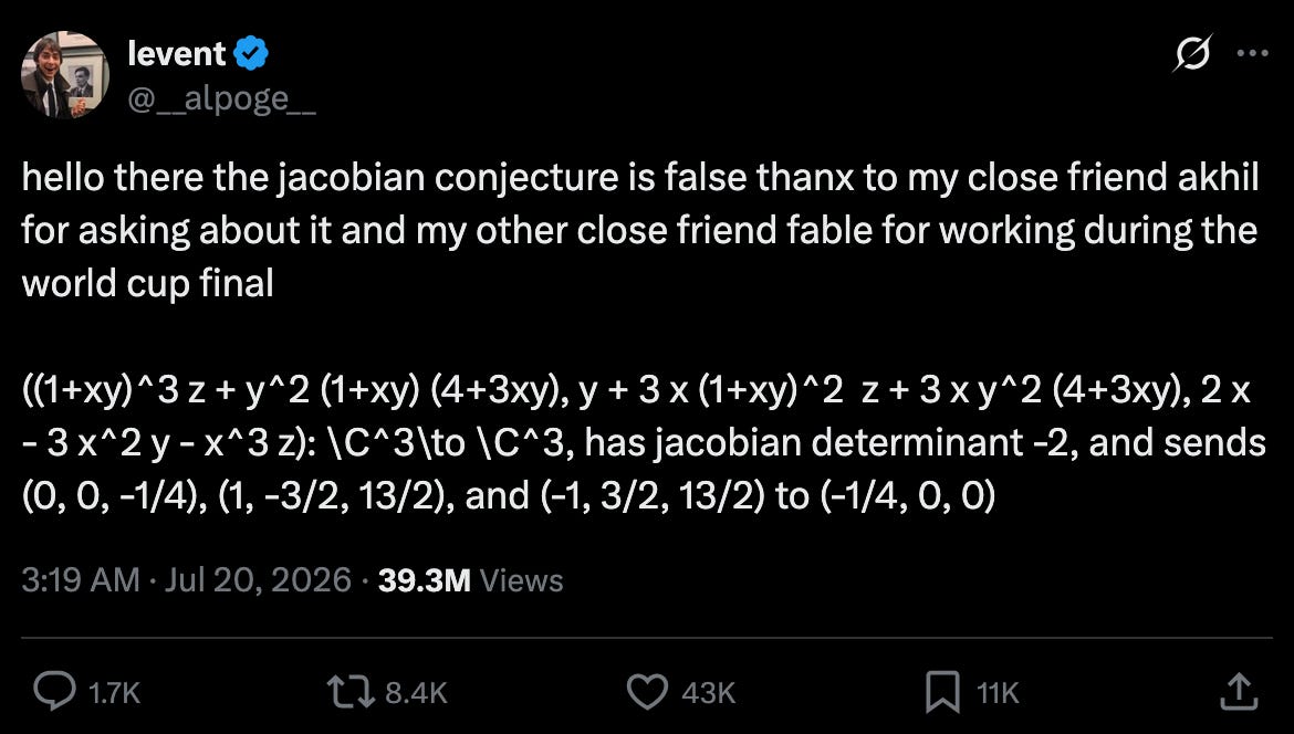
Take the recent mathematical proof – or rather disproof – of the Jacobian conjecture by Fable, announced on X:
It’s a remarkable finding, which has solved a puzzle that has frustrated mathematicians for decades. And in many ways, it’s the best in mathematical elegance and accessibility: a proof that can fit in a tweet and could be verified by any mathematics undergrad, or even a bright high school student.
Like many others, the first thing I did when I saw it was put the (x, y, z) co-ordinates into the equation to check it held up. But, like others, I then wondered how Fable had managed to spot such an elusive equation. And that’s where I hit a wall. It’s unlikely Fable found it by brute force alone – after all, humans have been trying for decades – but it’s still not clear exactly what it did behind the scenes.
What should one do?
Back in 1985, mathematician Jean-Pierre Serre expressed caution about the rise of proofs that ran to hundreds of pages, which hardly any humans could be expected to understand or check:
‘What should one do with such theorems, if one has to use them? Accept them on faith? Probably. But it is not a very comfortable situation.’
Serre was talking of proofs that were hard to verify. In contrast, AI proofs like the above are fairly easy to check. But the path the AI took to get there is often beyond reach. We have the what, but we frequently lack the why.
To paraphrase Serre: what should we do with such proofs?
In a recent talk, mathematician Terence Tao points out that there is more to mathematical research than just showing things are true:
For a proof to actually contribute to the broader field, it is not enough for it to be correct and easy to read. It also needs to be accepted and valued by the community. Other mathematicians need to digest the result and incorporate it into their own work.
Authors can assist in the digestion process by describing their own insights and stories from when they were working on the problem. However, current AI tools are quite opaque about their problem-solving process. This is particularly true for proprietary models whose inner workings remain a corporate secret.
Tao concluded with a suggestion that the ultimate goal of mathematical research is to have verified solutions that are ‘digested, accepted, and incorporated into the definitive theory of the field’.
Solved conjectures and stamp collecting
Nobel laureate Ernest Rutherford supposedly once said that ‘all science is either physics or stamp collecting’. In his view, the distinction came about because physics aimed to derive fundamental laws and mathematical principles, whereas other fields merely observe and categorise.
Many fields would rightly take issue with this generalisation, but the quote still came to my mind this week. Because I realised that I now knew a famous conjecture was false, but I didn’t have much beyond that.
Are we just collecting lots of little AI-proof-shaped stamps? In the long run, I expect it won’t be that simple. AI has the potential to show us a lot of things we’ve so far missed. But ‘show’ is the operative word here. It won’t be enough to tell us lots of things are true (or false); we’ll need the tales and theories that others can build on.